Change Point Detection Algorithm

Changepoint detection is the process of identifying when a data stream or time series shifts from one stable pattern to another, such as a sudden change in average temperature, a jump in stock prices, or a shift in a speaker’s pronunciation pattern. Instead of analyzing the entire dataset at once, changepoint detection works sequentially, monitoring data as it arrives and signaling when the underlying process likely changes. These shifts may reflect real-world events, system faults, or evolving behaviors.

Online Updating

To better understand the changepoint detection, let’s first introduce the idea of online updating.

How can we learn from data streams without storing or revealing everything?

We will use several activities to introduce the idea.

Welford’s Rule

Welford’s rule answers the question in terms of updating mean and variance by introducing the running mean \(\bar{X}_n\) .

\[ \bar{X}_1 = x_1 \]

\[ \bar{X}_2 = \frac{x_1+x_2}{2} = x_1 + \frac{x_2 - x_1}{2} =\bar{X}_1 + \frac{x_2 - \bar{X}_1}{2} \]

\[ .... \]

\[ \bar{X}_n = \frac{x_1 + ... + x_{n-1} + x_n}{n} = \frac{(n-1)\bar{X}_{n-1}+x_n}{n}= \bar{X}_{n-1} + \frac{x_n-\bar{X}_{n-1}}{n} \]

The running mean depends only on the previous sample average and the new observation, so it can be updated without recalculating from all raw data.

Can you derive the updating formula for

• Sample variance

• Likelihood Ratio

Adaptive Learning

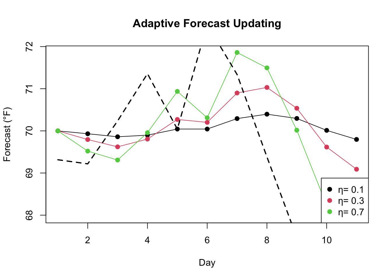
Adaptive learning refers to the idea that a system (or learner) continually updates its knowledge or predictions in response to new information, adjusting how much it learns each time based on experience or confidence. Instead of treating all data equally, adaptive learning assigns more weight to recent or reliable information and less to older or uncertain data, by choosing a different learning rate.

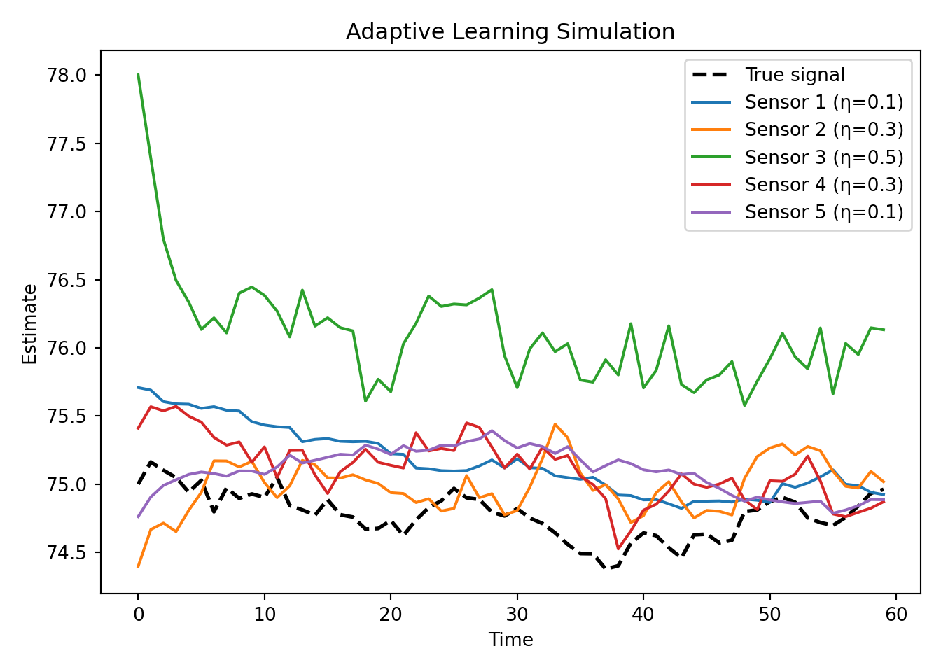
A sensor network is a connected system of multiple sensors that work together to monitor, measure, and share information about their environment. Each sensor collects local data, such as temperature, air quality, or vibration, and communicates with others or a central hub to form a more accurate and complete picture of the system being observed. It is popular to have adaptive learning in a sensor network.

Suppose \(x_i^t\) is the data observed by the \(i\)th sensor at time \(t\), then the estimate will be updated by

\[ x_i^{t+1} = (1-\eta) x_i^{t} + \eta \bar{x}^{t} \]

where \(\eta \in (0, 1)\) is the learning rate. Typical choices of \(\eta\):

• \(\eta = 0.1\) for slow learner;

• \(\eta = 0.3\) for moderate learner;

• \(\eta = 0.7\) for fast learner.

eta <- c(0.1, 0.3, 0.7)
true_temp <- 70 + cumsum(rnorm(10, 0, 1))  # slowly drifting true temp
f <- matrix(70, nrow = 3)                   # initial forecast

for (t in 1:(length(true_temp))) {
  f_next <- (1 - eta) * f[,t] + eta * true_temp[t]
  f <- cbind(f, f_next)
}

matplot(t(f), type="o", pch=19, col=1:3, lty=1,
        xlab="Day", ylab="Forecast (°F)", main="Adaptive Forecast Updating")
lines(true_temp, lty=2, lwd=2)
legend("bottomright", legend=paste("η=", eta), col=1:3, pch=19)

library("reticulate")

import numpy as np
import matplotlib.pyplot as plt
np.random.seed(1)

T = 60
theta = np.cumsum(np.r_[75, np.random.normal(0, 0.1, T-1)])  # slow drift
eta = np.array([0.1, 0.3, 0.5, 0.3, 0.1])
bias = np.array([0, 0, 2, 0, 0])
sd_noise = 0.8

x = np.empty((5, T))
x[:,0] = theta[0] + bias + np.random.normal(0, sd_noise, 5)

for t in range(T-1):
    net_avg = x[:,t].mean()
    y_t = theta[t] + bias + np.random.normal(0, sd_noise, 5)  # local noisy reading
    x[:,t+1] = (1-eta)*x[:,t] + eta*(0.5*net_avg + 0.5*y_t)

plt.figure()
plt.plot(theta, 'k--', linewidth=2, label='True signal')
for i in range(5):
    plt.plot(x[i], label=f'Sensor {i+1} (η={eta[i]:.1f})')
plt.xlabel('Time'); plt.ylabel('Estimate'); plt.title('Adaptive Learning Simulation')
plt.legend(); plt.tight_layout(); plt.show()

Adaptive learning shares the same idea with the Bayesian online updating:

\[ \text{New Estimate} = (1-\eta) \times \text{Old Estimate} + \eta \times \text{New Data} \]

What about the EWMA and CUSUM? Are these methods also using online updating?

Swinging Door Algorithm

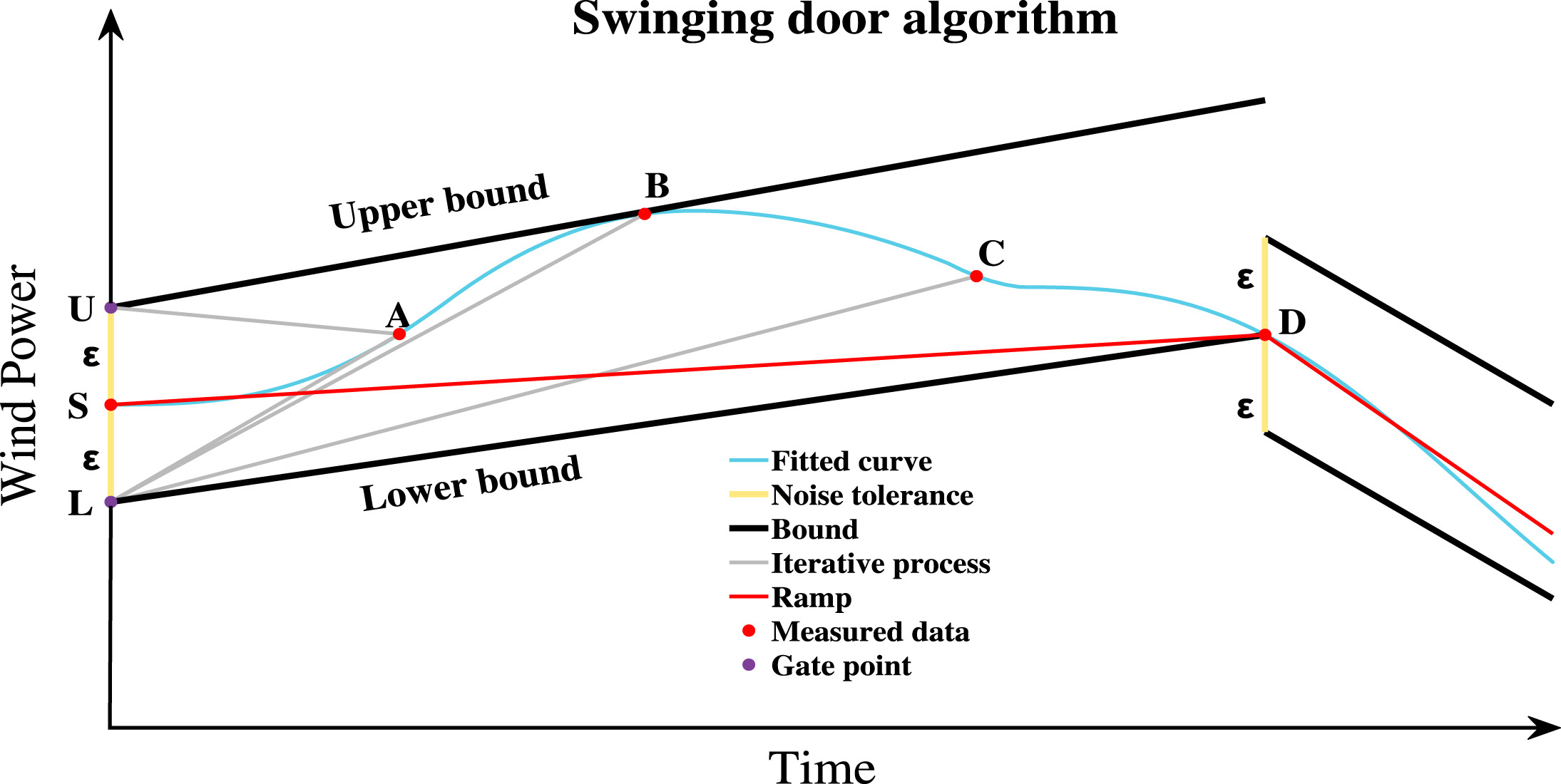
The Swinging Door Algorithm is a lossy down-sampling and compression algorithm for time-series or sequential data. It is designed for streaming or continuous monitoring data where huge numbers of data points are generated, but you don’t want to store every point if many of them lie along a nearly straight trend.

In essence, it monitors whether incoming data continue to lie within a “tolerance corridor” around an implied trend line;

• if they do, you skip storing them;

• if they diverge enough, you “close the door” (record the last point) and start a new segment.